Training

Training Dataset

For training, all image sets must be 512x512 and combined together in 3072x512 images (six images of size 512x512 stitched together horizontally). The data need to be arranged in the following order:

XXX_Dataset 
    ├── train
    └── val

We have provided a simple function in the CLI for preparing data for training.

• To prepare data for training, you need to have the image dataset for each image (including IHC, Hematoxylin Channel, mpIF DAPI, mpIF Lap2, mpIF marker, and segmentation mask) in the input directory. Each of the six images for a single image set must have the same naming format, with only the name of the label for the type of image differing between them. The label names must be, respectively: IHC, Hematoxylin, DAPI, Lap2, Marker, Seg. The command takes the address of the directory containing image set data and the address of the output dataset directory. It first creates the train and validation directories inside the given output dataset directory. It then reads all of the images in the input directory and saves the combined image in the train or validation directory, based on the given validation_ratio.

deepliif prepare-training-data --input-dir /path/to/input/images
                               --output-dir /path/to/output/images
                               --validation-ratio 0.2

Training

To train a model:

deepliif train --dataroot /path/to/input/images 
                --name Model_Name 

• To view training losses and results, open the URL http://localhost:8097. For cloud servers replace localhost with your IP.
• Epoch-wise intermediate training results are in DeepLIIF/checkpoints/Model_Name/web/index.html.
• Trained models will be by default be saved in DeepLIIF/checkpoints/Model_Name.
• Training datasets can be downloaded here.

Multi-GPU Training

There are 2 ways you can leverage multiple GPUs to train DeepLIIF, Data Parallel (DP) or Distributed Data Parallel (DDP). Both cases are a kind of data parallelism supported by PyTorch.

The key difference is that DP is single process multi-threading while DDP can have multiple processes.

TL;DR

Use DP if you - are used to the way to train DeepLIIF on multiple GPUs since its first release, OR - do not have multiple GPU machines to utilize, OR - are fine with the training being a bit slower

Use DDP if you - are willing to try a slightly different way to launch the training than before, OR - do have multiple GPU machines for cross-node distribution, OR - want to get as fast training as possible

Data Parallel (DP)

DP is single-process. It means that all the GPUs you want to use must be on the same machine so that they can be included in the same process - you cannot distribute the training across multiple GPU machines, unless you write your own code to handle inter-node (node = machine) communication.

To split and manage the workload for multiple GPUs within the same process, DP uses multi-threading.

It is worth noting that multi-threading in this case can lead to significant performance overhead, and slow down your training. See a short discussion in PyTorch's CUDA Best Practices.

Train with DP

Example with 2 GPUs (of course on 1 machine):

deepliif train --dataroot <data_dir> --batch-size 6 --gpu-ids 0 --gpu-ids 1

Note that

1. batch-size is defined per process. Since DP is a single-process method, the batch-size you set is the effective batch size.

Distributed Data Parallel (DDP)

DDP usually spawns multiple processes.

DeepLIIF's code follows the PyTorch recommendation to spawn 1 process per GPU (doc). If you want to assign multiple GPUs to each process, you will need to make modifications to DeepLIIF's code (see doc).

Despite all the benefits of DDP, one drawback is the extra GPU memory needed for dedicated CUDA buffer for communication. See a short discussion here. In the context of DeepLIIF, this means that there might be situations where you could use a bigger batch size with DP as compared to DDP, which may actually train faster than using DDP with a smaller batch size.

Train with DDP

1. Local Machine

To launch training using DDP on a local machine, use deepliif trainlaunch. Example with 2 GPUs (on 1 machine):

deepliif trainlaunch --dataroot <data_dir> --batch-size 3 --gpu-ids 0 --gpu-ids 1 --use-torchrun "--nproc_per_node 2"

Note that

1. batch-size is defined per process. Since DDP is a single-process method, the batch-size you set is the batch size for each process, and the effective batch size will be batch-size multiplied by the number of processes you started. In the above example, it will be 3 * 2 = 6.
2. You still need to provide all GPU ids to use to the training command. Internally, in each process DeepLIIF picks the device using gpu_ids[local_rank]. If you provide --gpu-ids 2 --gpu-ids 3, the process with local rank 0 will use gpu id 2 and that with local rank 1 will use gpu id 3.

3. -t 3 --log_dir <log_dir> is not required, but is a useful setting in torchrun that saves the log from each process to your target log directory. For example:

   deepliif trainlaunch --dataroot <data_dir> --batch-size 3 --gpu-ids 0 --gpu-ids 1 --use-torchrun "-t 3 --log_dir <log_dir> --nproc_per_node 2"

4. If your PyTorch is older than 1.10, DeepLIIF calls torch.distributed.launch in the backend. Otherwise, DeepLIIF calls torchrun.

2. Kubernetes-Based Training Service

To launch training using DDP on a kubernetes-based service where each process will have its own pod and a dedicated GPU, and there is an existing task manager/scheduler in place, you may submit a script with training command like the following:

import os
import torch.distributed as dist
def init_process():
    dist.init_process_group(
        backend='nccl',
        init_method='tcp://' + os.environ['MASTER_ADDR'] + ':' + os.environ['MASTER_PORT'],
        rank=int(os.environ['RANK']),
        world_size=int(os.environ['WORLD_SIZE']))

root_folder = <data_dir>

if __name__ == '__main__':
    init_process()
    subprocess.run(f'deepliif train --dataroot {root_folder} --remote True --batch-size 3 --gpu-ids 0',shell=True)

Note that

1. Always provide --gpu-ids 0 to the training command for each process/pod if the gpu id gets re-named in each pod. If not, you will need to pass the correct gpu id in a dynamic way, possibly through an environment variable in each pod.

3. Multiple Virtual Machines

To launch training across multiple VMs, you can refer to the scheduler framework you use. For each process, similar to the example for kubernetes, you will need to initiate the process group so that the current process knows who it is, where are its peers, etc., and then execute the regular training command in a subprocess.

Move from Single-GPU to Multi-GPU: Impact on Hyper-Parameters

To achieve equivalently good training results, you may want to adjust some hyper-parameters you figured out for a single GPU training.

Batch Size & Learning Rate

Backward propagation by default runs at the end of every batch to find how much change to make in parameters. An immediate outcome from using multiple GPUs is that we have a larger effective batch size.

In DDP, this means fewer gradient descent because DDP averages the gradients from all processes (doc). Assume that in 1 epoch, a single-GPU training does gradient descent for 200 times. Now with 2 GPUs/processes, the training will have 100 batches in each process and does the gradient descent using the averaged gradients of the 2 GPUs/processes, one for each batch, which is 100 times.

You may want to compensate this by increasing the learning rate proportionally.

DP is slightly different, in that it sums up the gradients from all GPUs/threads (doc). However, practically the performance (accuracy) still suffers from the larger effective batch size, which can be mitigated by increasing the learning rate.

Track Training Progress in Visualizer

When using multiple GPUs for training, tracking training progress in the visdom visualizer can be tricky. It may not be a big issue for DP which uses only 1 process, but definitely the multi-processing in DDP brings a challenge.

With DDP, each process trains on its own slice of data that is different from the others. If we plot the training progress from the processes in terms of losses, the raw values will not be comparable, and you will see a different graph from each process. These graphs might be close, but will not be exactly the same.

Currently, if you use multiple processes (DDP), you are suggested to:

1. pass --remote True to the training command, even if you are running on a local machine

2. open a terminal in an environment you intend to have visdom running (it can be the same place where you train the model, or a separate machine), and run deepliif visualize:

   deepliif visualize --pickle_dir <pickle_dir>

By default, the pickle files are stored under <checkpoint_dir_in_training_command>/<name_in_training_command>/pickle.

--remote True in the training command triggers DeepLIIF to i) not start a visdom session and ii) persist the input into the visdom graphs as pickle files. If there are multiple processes, it will only persist the information such as losses from the first process (process with rank 0). The visualize command deepliif visualize then starts the visdom, scans the pickle directory you provided periodically, and updates the graphs if there is an update in any pickled snapshot.

If you plan to train the model in a different place from where you would like to host visdom (e.g., situation 2 & 3 in DDP mentioned above), you need to make sure that this pickle directory is accessible by both the training environment and the visdom environment. For example:

• use a storage volume mounted to both environments, so you can access this storage simply using a file path
• use an external storage of your choice

For training

1. write a script that contains one function DeepLIIF can call to transfer the files like the following:

import boto3

credentials = <s3 credentials>

# make sure that the first argument is the source path
def save_to_s3(source_path):
# make sure the file name part is still unchanged, e.g., by keeping source_path.split('/')[-1]
target_path = ... 

s3 = boto3.client('s3')
with open(source_path, "rb") as f:
    s3.upload_fileobj(f, credentials["bucket_name"], target_path)

2. save it in a directory where you will call the training command; let's say the script is called mysave.py

3. tell DeepLIIF to use this by passing --remote-transfer-cmd mysave.save_to_s3 to the training command (take kubernetes-based training service as an example):

import os
import torch.distributed as dist
def init_process():
    dist.init_process_group(
        backend='nccl',
        init_method='tcp://' + os.environ['MASTER_ADDR'] + ':' + os.environ['MASTER_PORT'],
        rank=int(os.environ['RANK']),
        world_size=int(os.environ['WORLD_SIZE']))

root_folder = <data_dir>

if __name__ == '__main__':
    init_process()
    subprocess.run(f'deepliif train --dataroot {root_folder} --remote True --batch-size 3 --gpu-ids 0 --remote True, --remote-transfer-cmd mysave.save_to_s3',shell=True)

• note that this method if used will be applied not only on the pickled snapshots for visdom input, but also the model files DeepLIIF saves: DeepLIIF will trigger this provided method to store an additional copy of the model files into your external storage

For visualization

1. periodically check and download the latest pickle files from your external storage to your local environment
2. pass the pickle directory in your local enviroment to deepliif visualize

Synthetic Data Generation

The first version of DeepLIIF model suffered from its inability to separate IHC positive cells in some large clusters, resulting from the absence of clustered positive cells in our training data. To infuse more information about the clustered positive cells into our model, we present a novel approach for the synthetic generation of IHC images using co-registered data. We design a GAN-based model that receives the Hematoxylin channel, the mpIF DAPI image, and the segmentation mask and generates the corresponding IHC image. The model converts the Hematoxylin channel to gray-scale to infer more helpful information such as the texture and discard unnecessary information such as color. The Hematoxylin image guides the network to synthesize the background of the IHC image by preserving the shape and texture of the cells and artifacts in the background. The DAPI image assists the network in identifying the location, shape, and texture of the cells to better isolate the cells from the background. The segmentation mask helps the network specify the color of cells based on the type of the cell (positive cell: a brown hue, negative: a blue hue).

In the next step, we generate synthetic IHC images with more clustered positive cells. To do so, we change the segmentation mask by choosing a percentage of random negative cells in the segmentation mask (called as Neg-to-Pos) and converting them into positive cells. Some samples of the synthesized IHC images along with the original IHC image are shown below.

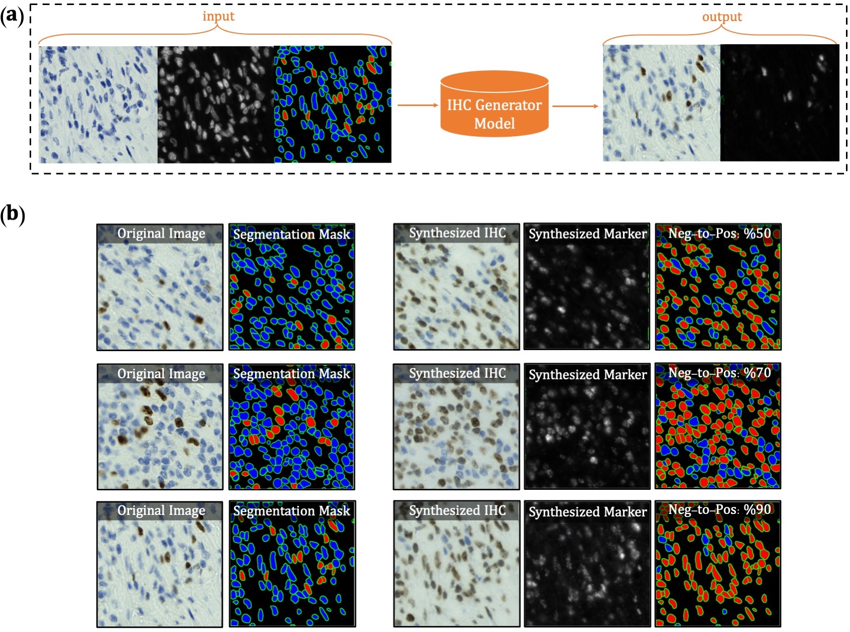Overview of synthetic IHC image generation. (a) A training sample of the IHC-generator model. (b) Some samples of synthesized IHC images using the trained IHC-Generator model. The Neg-to-Pos shows the percentage of the negative cells in the segmentation mask converted to positive cells.

We created a new dataset using the original IHC images and synthetic IHC images. We synthesize each image in the dataset two times by setting the Neg-to-Pos parameter to %50 and %70. We re-trained our network with the new dataset. You can find the new trained model here.

Registration

To register the de novo stained mpIF and IHC images, you can use the registration framework in the 'Registration' directory. Please refer to the README file provided in the same directory for more details.

Contributing Training Data

To train DeepLIIF, we used a dataset of lung and bladder tissues containing IHC, hematoxylin, mpIF DAPI, mpIF Lap2, and mpIF Ki67 of the same tissue scanned using ZEISS Axioscan. These images were scaled and co-registered with the fixed IHC images using affine transformations, resulting in 1667 co-registered sets of IHC and corresponding multiplex images of size 512x512. We randomly selected 709 sets for training, 358 sets for validation, and 600 sets for testing the model. We also randomly selected and segmented 41 images of size 640x640 from recently released BCDataset which contains Ki67 stained sections of breast carcinoma with Ki67+ and Ki67- cell centroid annotations (for cell detection rather than cell instance segmentation task). We split these tiles into 164 images of size 512x512; the test set varies widely in the density of tumor cells and the Ki67 index. You can find this dataset here.

We are also creating a self-configurable version of DeepLIIF which will take as input any co-registered H&E/IHC and multiplex images and produce the optimal output. If you are generating or have generated H&E/IHC and multiplex staining for the same slide (de novo staining) and would like to contribute that data for DeepLIIF, we can perform co-registration, whole-cell multiplex segmentation via ImPartial, train the DeepLIIF model and release back to the community with full credit to the contributors.